[엑셀 함수]HLOOUP과 VLOOKUP에 대하여 알아봅시다
Excel은 데이터를 관리하고 분석하는 강력한 도구입니다. 엑셀에서 사용할 수 있는 많은 기능 중에서 VLOOKUP과 HLOOKUP은 가장 유용하고 일반적으로 사용되는 기능입니다. 이러한 함수를 사용하여 테이블에서 특정 값을 검색하고 위치를 기반으로 정보를 검색할 수 있습니다. 이번 블로그 게시물에서는 VLOOKUP 및 HLOOKUP에 대해 자세히 살펴보고 Excel에서 사용할 수 있는 방법에 대해 알아보겠습니다.
VLOOKUP - 수직 조회

VLOOKUP은 "Vertical Lookup"를 나타내며 테이블의 맨 왼쪽 열에서 값을 검색하고 동일한 행의 다른 열에서 정보를 검색하는 데 사용됩니다. 이 기능은 대규모 데이터셋을 사용할 때 특히 유용하며 특정 기준에 따라 정보를 신속하게 검색해야 합니다.
VLOOKUP의 구문은 다음과 같습니다:
=VLOOKUP(lookup_value, table_array, col_index_num, [range_value])

Lookup_value: 표의 맨 왼쪽 열에서 검색할 값입니다.
테이블_array: 검색할 테이블이 포함된 셀 범위입니다.
Col_index_num: 검색할 정보가 들어 있는 테이블의 열 번호(1부터 시작).
Range_lookup: 정확한 일치(FALSE) 또는 근사 일치(TRUE) 중 어느 것을 원하는지 지정하는 선택적 매개 변수입니다. 생략할 경우 기본값은 TRUE입니다.
예를 들어 직원의 이름, ID 번호 및 급여가 나열된 표가 있다고 가정합니다. ID 번호를 기준으로 특정 직원의 급여를 찾으려고 합니다. VLOOKUP을 사용하여 테이블의 맨 왼쪽 열에서 ID 번호를 검색하고 해당 행에서 급여를 검색할 수 있습니다.
HLOOKUP - 수평 조회

HLOOKUP은 "Horizontal Lookup"을 나타내며 테이블의 맨 위 행에서 값을 검색하고 동일한 열의 다른 행에서 정보를 검색하는 데 사용됩니다. 이 기능은 특정 범주 또는 레이블을 기준으로 정보를 검색해야 할 때 유용합니다.
HLOOKUP의 구문은 다음과 같습니다:
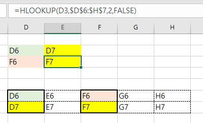
=HLOOKUP(lookup_value, table_array, row_index_num, [range_message])
Lookup_value: 표의 맨 위 행에서 검색할 값입니다.
테이블_array: 검색할 테이블이 포함된 셀 범위입니다.
row_index_num: 검색할 정보가 들어 있는 테이블의 행 번호(1부터 시작).
Range_lookup: 정확한 일치(FALSE) 또는 근사 일치(TRUE) 중 어느 것을 원하는지 지정하는 선택적 매개 변수입니다. 생략할 경우 기본값은 TRUE입니다.
예를 들어 도시 이름, 연도 및 인구가 나열된 표가 있다고 가정합니다. 연도를 기준으로 특정 도시의 인구를 찾으려고 합니다. HLOOKUP을 사용하여 표의 맨 위 행에서 연도를 검색하고 해당 열에서 모집단을 검색할 수 있습니다.
VLOOKUP 및 HLOOKUP 사용 팁
다음은 VLOOKUP 및 HLOOKUP을 사용할 때 참고해야 할 몇 가지 팁입니다:
룩업 값이 테이블의 맨 왼쪽 열 또는 맨 위 행에서 고유한지 확인합니다. 중복 항목이 있는 경우 함수는 처음 찾은 일치 항목만 반환합니다.
col_index_num 또는 row_index_num 인수는 검색할 정보가 들어 있는 열 또는 행의 수를 나타내는 양의 정수여야 합니다.
정확한 일치를 사용할지 또는 대략적인 일치를 사용할지 확신할 수 없는 경우 FALSE를 사용하여 정확한 일치를 확인합니다. 이것은 수치 데이터를 다루거나 데이터를 특정 순서로 정렬할 때 특히 중요합니다.
(Eng. Ver)
Excel is a powerful tool for managing and analyzing data. Among the many functions available in Excel, VLOOKUP and HLOOKUP are two of the most useful and commonly used. These functions allow you to search for a specific value in a table and retrieve information based on its location. In this blog post, we'll take a closer look at VLOOKUP and HLOOKUP and how they can be used in Excel.
VLOOKUP - Vertical Lookup

VLOOKUP stands for "Vertical Lookup" and is used to search for a value in the leftmost column of a table and retrieve information from other columns of the same row. This is particularly useful when working with large datasets and you need to quickly retrieve information based on a specific criteria.
The syntax for VLOOKUP is as follows:
=VLOOKUP(lookup_value, table_array, col_index_num, [range_lookup])
Lookup_value: The value you want to search for in the leftmost column of the table.
Table_array: The range of cells that contains the table you want to search.
Col_index_num: The column number (starting from 1) of the table that contains the information you want to retrieve.
Range_lookup: Optional parameter that specifies whether you want an exact match (FALSE) or an approximate match (TRUE). If omitted, the default value is TRUE.
For example, suppose you have a table that lists the names of employees, their ID numbers, and their salaries. You want to find the salary of a specific employee based on their ID number. You can use VLOOKUP to search for the ID number in the leftmost column of the table and retrieve the salary from the corresponding row.
HLOOKUP - Horizontal Lookup

HLOOKUP stands for "Horizontal Lookup" and is used to search for a value in the top row of a table and retrieve information from other rows of the same column. This is useful when you need to retrieve information based on a specific category or label.
The syntax for HLOOKUP is as follows:
=HLOOKUP(lookup_value, table_array, row_index_num, [range_lookup])
Lookup_value: The value you want to search for in the top row of the table.
Table_array: The range of cells that contains the table you want to search.
Row_index_num: The row number (starting from 1) of the table that contains the information you want to retrieve.
Range_lookup: Optional parameter that specifies whether you want an exact match (FALSE) or an approximate match (TRUE). If omitted, the default value is TRUE.
For example, suppose you have a table that lists the names of cities, the year, and the population. You want to find the population of a specific city based on the year. You can use HLOOKUP to search for the year in the top row of the table and retrieve the population from the corresponding column.
Tips for Using VLOOKUP and HLOOKUP
Here are some tips to keep in mind when using VLOOKUP and HLOOKUP:
Make sure that the lookup value is unique in the leftmost column or top row of the table. If there are duplicates, the function will only return the first match it finds.
The col_index_num or row_index_num argument should be a positive integer that represents the number of the column or row that contains the information you want to retrieve.
If you're not sure whether to use an exact match or an approximate match, use FALSE to ensure that you get an exact match. This is particularly important when dealing with numerical data or when the data is sorted in a specific order.